A Three tank example
This is a slightly larger example on residual generator design/simulation for the Three-tank example from the paper
“Diagnosability Analysis Considering Causal Interpretations for Differential Constraints”, Erik Frisk, Anibal Bregon, Jan Aaslund, Mattias Krysander, Belarmino Pulido, and Gautam Biswas IEEE Transactions on Systems, Man and Cybernetics, Part A: Systems and Humans (2012), Vol. 42, No. 5, 1216-1229.

This example will go through the process of * defining a model * initial model analysis * residual generator analysis * generating C-code for a few residual generators * simulating the process and generating synthetic data * running the residual generators on the generated data
First, the necessary imports
[35]:
import faultdiagnosistoolbox as fdt
import sympy as sym
import numpy as np
import matplotlib.pyplot as plt
from scipy.linalg import solve_continuous_are
import seaborn as sns
import os
import TankSimulation
Defining the model
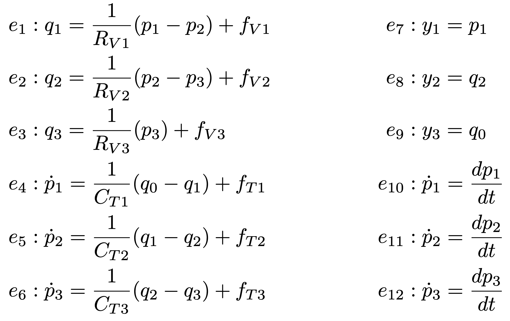
The model is a simple, linear, model in 12 equations, with threee measurements, and 6 faults as below
Using the symbolic toolbox sympy, the model can be defined by
[36]:
modelDef = {}
modelDef['type'] = 'Symbolic'
modelDef['x'] = ['p1', 'p2', 'p3', 'q0', 'q1', 'q2', 'q3', 'dp1', 'dp2', 'dp3']
modelDef['f'] = ['fV1', 'fV2', 'fV3', 'fT1', 'fT2', 'fT3']
modelDef['z'] = ['y1', 'y2', 'y3']
modelDef['parameters'] = ['Rv1', 'Rv2', 'Rv3', 'CT1', 'CT2', 'CT3']

p1, p2, p3, q0, q1, q2, q3, dp1, dp2, dp3 = sym.symbols(modelDef['x'])
fV1, fV2, fV3, fT1, fT2, fT3 = sym.symbols(modelDef['f'])
y1, y2, y3 = sym.symbols(modelDef['z'])
Rv1, Rv2, Rv3, CT1, CT2, CT3 = sym.symbols(modelDef['parameters'])

modelDef['rels'] = [
    -q1 + 1 / Rv1 * (p1 - p2) + fV1,
    -q2 + 1 / Rv2 * (p2 - p3) + fV2,
    -q3 + 1 / Rv3 * p3 + fV3,
    -dp1 + 1 / CT1 * (q0 - q1) + fT1,
    -dp2 + 1 / CT2 * (q1 - q2) + fT2,
    -dp3 + 1 / CT3 * (q2 - q3) + fT3,
    -y1 + p1, -y2 + q2, -y3 + q0,
    fdt.DiffConstraint('dp1', 'p1'),
    fdt.DiffConstraint('dp2', 'p2'),
    fdt.DiffConstraint('dp3', 'p3')]

model = fdt.DiagnosisModel(modelDef, name='Three Tank System')
model_params = {'Rv1': 1, 'Rv2': 1, 'Rv3': 1, 'CT1': 1, 'CT2': 1, 'CT3': 1}

model.Lint()
Model: Three Tank System

  Type:Symbolic, dynamic

  Variables and equations
    10 unknown variables
    3 known variables
    6 fault variables
    12 equations, including 3 differential constraints

  Degree of redundancy: 2
  Degree of redundancy of MTES set: 1


  Model validation finished with 0 errors and 0 warnings.
The model structure can be visualized as
[37]:
_, ax = plt.subplots(num=10, clear=True)
model.PlotModel()

Initial model analysis
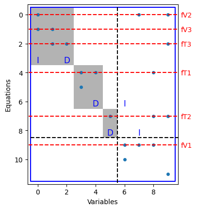
A basic Dulmage-Mendelsohn decoposition illustrates isolability properties of the model
[38]:
_, ax = plt.subplots(num=23, clear=True)
model.PlotDM(ax=ax, fault=True, eqclass=True)
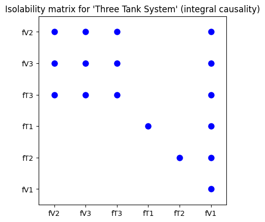
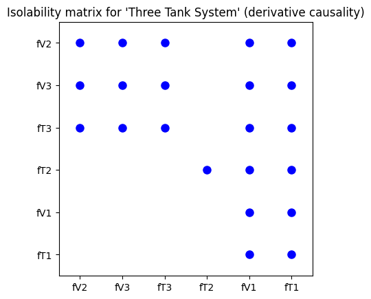
A more detailed isolability analysis, considering different causality assumptions can be done using the IsolabilityAnalysis class method
[39]:
_, ax = plt.subplots(num=20, clear=True)
model.IsolabilityAnalysis(ax=ax)

_, ax = plt.subplots(num=21, clear=True)
model.IsolabilityAnalysis(ax=ax, causality='int')

_, ax = plt.subplots(num=22, clear=True)
_ = model.IsolabilityAnalysis(ax=ax, causality='der')

Residual generator analysis
First, compute the set of MSO and MTES sets
[40]:
msos = model.MSO()
mtes = model.MTES()
print(f"Found {len(msos)} MSO sets")
print(f"Found {len(mtes)} MTES sets")
Found 6 MSO sets
Found 4 MTES sets
Look at differential-index properties of the MSO and MTES sets
[41]:
li_msos = [m for m in msos if model.IsLowIndex(m)]
li_mtes = [m for m in mtes if model.IsLowIndex(m)]
print(f"{len(li_msos)} of the MSO sets are low index")
print(f"{len(li_mtes)} of the MTES sets are low index")
5 of the MSO sets are low index
3 of the MTES sets are low index
Take two MSO sets with different index properties and see how to choose redundant equations
[42]:
mso1 = msos[0]
mso2 = msos[1]
print(model.MSOCausalitySweep(mso1))
print(model.MSOCausalitySweep(mso2))
['mixed', 'mixed', 'mixed', 'mixed', 'mixed', 'mixed', 'mixed', 'mixed', 'mixed', 'mixed', 'mixed']
['der', 'int', 'der', 'mixed', 'mixed', 'mixed', 'int', 'mixed']
Here it is clear that in mso1, no choice of residual equation gives integral causality in the residual generator. However, for mso2, two equations are possible!
Residual generator design and code generation
Now, three residual generators will be designed corresponding to figures 2, 3, and 12 in the paper.
Residuals, code generation
Residual 1 is based on the second MSO set, using equation e5 as a redundant equation, which will result in a sequential residual generator in derivative causality. The computational graph, Fig. 2 in the paper, is given by:
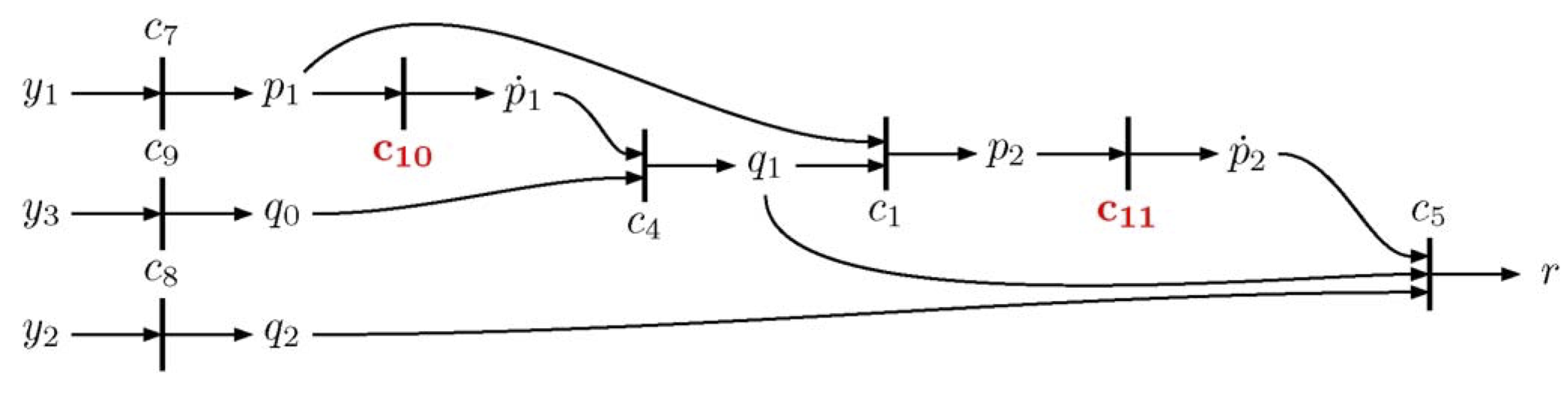
[43]:
eqr1 = mso2
redeq1 = 4
m01 = [e for e in eqr1 if e != redeq1]
Gamma1 = model.Matching(m01)
model.SeqResGen(Gamma1, redeq1, 'ResGen1', batch=True, language='C')
print("")
Generating residual generator ResGen1 (C, batch)
  Generating code for the exactly determined part: .......
  Generating code for the residual equations
  Writing residual generator file
Files ResGen1.cc and ResGen1_setup.py generated
Compile by running: python ResGen1_setup.py build_ext --inplace
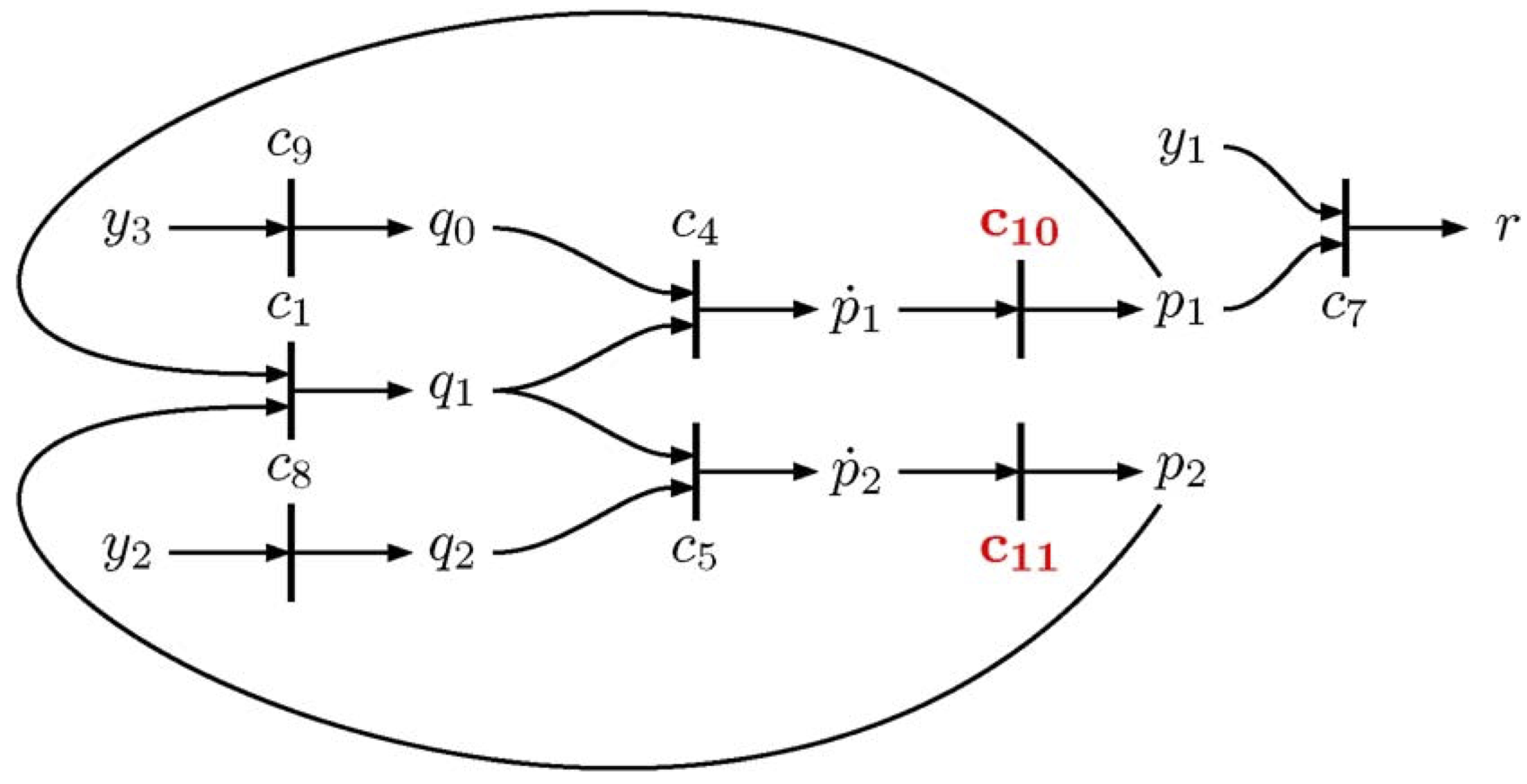
Residual 2 is based on the same second MSO set but using equation e7 as a redundant equation, which will result in a sequential residual generator in integral causality. The computational graph, Fig. 3 in the paper, is given by:
[44]:
eqr2 = mso2
redeq2 = 6
m02 = [e for e in eqr2 if e != redeq2]
Gamma2 = model.Matching(m02)
model.SeqResGen(Gamma2, redeq2, 'ResGen2', batch=True, language='C')
print("")
Generating residual generator ResGen2 (C, batch)
  Generating code for the exactly determined part: ...
  Generating code for the residual equations
  Writing residual generator file
Files ResGen2.cc and ResGen2_setup.py generated
Compile by running: python ResGen2_setup.py build_ext --inplace
Residual 3 is based on the first MSO set using equation e2 as a redundant equation, which will result in a sequential residual generator in mixed causality. The computational graph, Fig. 12 in the paper, is given by:
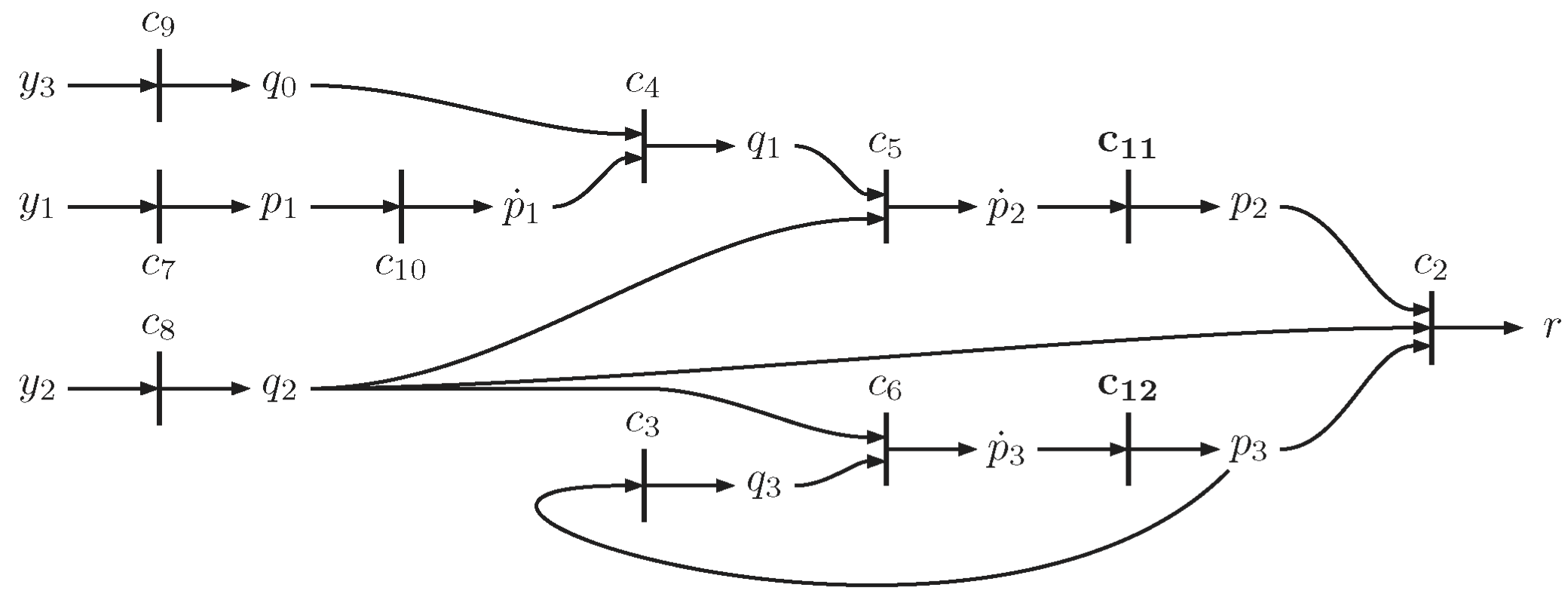
[45]:
eqr3 = mso1
redeq3 = 1
m03 = [e for e in eqr3 if e != redeq3]
Gamma3 = model.Matching(m03)
model.SeqResGen(Gamma3, redeq3, 'ResGen3', batch=True, language='C')
print("")
Generating residual generator ResGen3 (C, batch)
  Generating code for the exactly determined part: ........
  Generating code for the residual equations
  Writing residual generator file
Files ResGen3.cc and ResGen3_setup.py generated
Compile by running: python ResGen3_setup.py build_ext --inplace
Residuals, compile generated code
Now that the code is generated, compile and import the generated c-extension modules.
[46]:
for resName in ['ResGen1', 'ResGen2', 'ResGen3']:
    print(f"Compiling residual generator: {resName} ... ", end='')
    compile_cmd = f"python {resName}_setup.py build_ext --inplace > /dev/null"
    if os.system(compile_cmd) == 0:
        print('Success!')
    else:
        print('Failure!')
Compiling residual generator: ResGen1 ... Success!
Compiling residual generator: ResGen2 ... Success!
Compiling residual generator: ResGen3 ... Success!
and import
[47]:
import ResGen1
import ResGen2
import ResGen3
print("All residual generators imported/reloaded")
All residual generators imported/reloaded
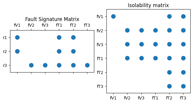
Diagnosis properties of the three generated residuals
Generate the fault signature matrix (FSM) and isolability properties of the three generated residual generators.
[48]:
_, ax = plt.subplots(1, 2, num=50, clear=True, layout="constrained")
FSM = model.FSM([mso2, mso2, mso1])
ax[0].spy(FSM, markersize=10, marker="o")
ax[0].set_yticks(range(3))
ax[0].set_yticklabels([f"r{k + 1}" for k in range(3)])
ax[0].set_xticks(range(6))
ax[0].set_xticklabels(model.f)
ax[0].set_title('Fault Signature Matrix')

model.IsolabilityAnalysisFSM(FSM, ax=ax[1])
ax[1].set_title('Isolability matrix')
[48]:
Text(0.5, 1.0, 'Isolability matrix')
Simulate
Next step is to simulate the process with all faults. For this, we need a controller. Here, a simple LQR-controller is designed to follow a reference pressure in the first tank.
[49]:
G = TankSimulation.ThreeTank_ss(model_params)  # Get state-space matrices

Q = np.eye(3)
R = np.eye(1) * 0.5
P = solve_continuous_are(G['A'], G['B'], Q, R)
Lx = np.linalg.solve(R, G['B'].T @ P)
Lr = -1 / (np.array([1, 0, 0]) @ np.linalg.inv(G['A'] - G['B'] @ Lx) @ G['B'])
Define the reference signal and the controller function
[50]:
def ref(t):
    return 0.2 * np.sin(2 * np.pi * 1 / 10 * t) + 1


def controller(t, x):
    return (-Lx @ x + Lr * ref(t))[0]
Now, simulate the fault-free behavior and all 6 fault modes. For each fault mode, a ramp-function is used as the fault signal.
[51]:
t = np.linspace(0, 20, 201)
x0 = [0, 0, 0]
sim = ({'NF': TankSimulation.SimScenario(0, lambda t: 0 * t, controller, model_params, t, x0)} |
       {fi: TankSimulation.SimScenario(k + 1, lambda t: 0.3 * TankSimulation.ramp(t, 6, 10), controller, model_params, t, x0) for k, fi in enumerate(model.f)})
Plot some data from the fault-free and the fV1 scenarios
[52]:
_, ax = plt.subplots(3, 2, num=40, clear=True, layout="constrained")
ax[0, 0].plot(sim['NF'].t, sim['NF'].w[0], 'b', label='p1')
ax[0, 0].plot(sim['NF'].t, ref(sim['NF'].t), 'b--', label='p1ref')
ax[0, 0].plot(sim['NF'].t, sim['NF'].w[1], 'r', label='p2')
ax[0, 0].plot(sim['NF'].t, sim['NF'].w[2], 'g', label='p3')
ax[0, 0].set_ylabel('Tank water pressure')
ax[0, 0].set_title('Fault free simulation')
sns.despine(ax=ax[0, 0])

ax[1, 0].plot(sim['NF'].t, sim['NF'].w[3])
ax[1, 0].set_ylabel('q0')
sns.despine(ax=ax[1, 0])

ax[2, 0].plot(sim['NF'].t, sim['NF'].f)
ax[2, 0].set_ylabel('Fault signal')
ax[2, 0].set_xlabel('t [s]')
sns.despine(ax=ax[2, 0])

ax[0, 1].plot(sim['fV1'].t, sim['fV1'].w[0], 'b', label='p1')
ax[0, 1].plot(sim['fV1'].t, ref(sim['fV1'].t), 'b--', label='p1ref')
ax[0, 1].plot(sim['fV1'].t, sim['fV1'].w[1], 'r', label='p2')
ax[0, 1].plot(sim['fV1'].t, sim['fV1'].w[2], 'g', label='p3')
ax[0, 1].set_ylabel('Tank water pressure')
ax[0, 1].legend(loc='upper right', bbox_to_anchor=(1.5, 1.0))
ax[0, 1].set_title('Fault scenario Fv1')
sns.despine(ax=ax[0, 1])

ax[1, 1].plot(sim['fV1'].t, sim['fV1'].w[3])
ax[1, 1].set_ylabel('q0')
sns.despine(ax=ax[1, 1])

ax[2, 1].plot(sim['fV1'].t, sim['fV1'].f)
ax[2, 1].set_ylabel('Fault signal')
ax[2, 1].set_xlabel('t [s]')
sns.despine(ax=ax[2, 1])

Run residual generators on simulated data
Run the three residual generators on all generated data
[53]:
res = {}
for fault_mode in ['NF'] + model.f:
    Ts = sim[fault_mode].t[1] - sim[fault_mode].t[0]

    state1 = {'p1': sim[fault_mode].w[0, 0], 'p2': sim[fault_mode].w[1, 0]}
    state2 = {'p1': sim[fault_mode].w[0, 0], 'p2': sim[fault_mode].w[1, 0]}
    state3 = {'p1': sim[fault_mode].w[0, 0], 'p2': sim[fault_mode].w[1, 0], 'p3': sim[fault_mode].w[2, 0]}

    r1 = ResGen1.ResGen1(sim[fault_mode].z, state1, model_params, Ts)
    r2 = ResGen2.ResGen2(sim[fault_mode].z, state2, model_params, Ts)
    r3 = ResGen3.ResGen3(sim[fault_mode].z, state3, model_params, Ts)
    r1[0:2] = 0.0
    r3[0] = 0.0
    res[fault_mode] = np.row_stack((r1, r2, r3))
and plot some results
[54]:
# Plot some results
fig, ax = plt.subplots(3, 1, num=60, clear=True, layout="constrained")
for fault_mode in res:
    ax[0].plot(sim[fault_mode].t, res[fault_mode][0], label=fault_mode)
    ax[1].plot(sim[fault_mode].t, res[fault_mode][1])
    ax[2].plot(sim[fault_mode].t, res[fault_mode][2])
sns.despine(ax=ax[0])
ax[0].legend(bbox_to_anchor=(1.05, 1))
ax[0].set_title('r1 (seq/derivative/discrete)')
sns.despine(ax=ax[1])
ax[1].set_title('r2 (seq/integral/discrete)')
sns.despine(ax=ax[2])
ax[2].set_title('r3 (seq/mixed/discrete)')
[54]:
Text(0.5, 1.0, 'r3 (seq/mixed/discrete)')
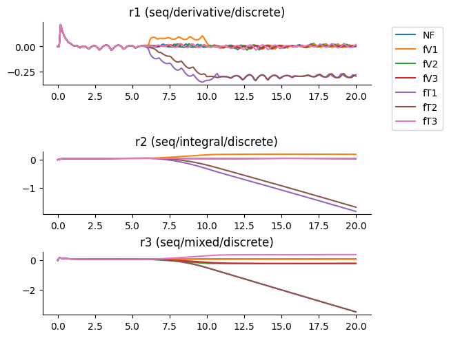
Here it is clear that the residual with numerical differentiation is unreliable and requres additional filtering.