Small induction motor example

Illustrating basic functionality on a small induction motor example. The model equations are taken from the paper

Aguilera, F., et al. “Current-sensor fault detection and isolation for induction-motor drives using a geometric approach.”, Control Engineering Practice 53 (2016): 35-46.

import matplotlib.pyplot as plt
import faultdiagnosistoolbox as fdt
import sympy as sym

Modelling

First, define the model using the sympy symbolic toolbox in Python.

model_def = {'type': 'Symbolic',
             'x': ['i_a', 'i_b', 'lambda_a', 'lambda_b', 'w',
                   'di_a', 'di_b', 'dlambda_a', 'dlambda_b', 'dw', 'q_a', 'q_b', 'Tl'],
             'f': ['f_a', 'f_b'], 'z': ['u_a', 'u_b', 'y1', 'y2', 'y3'],
             'parameters': ['a', 'b', 'c', 'd', 'L_M', 'k', 'c_f', 'c_t']}

i_a, i_b, lambda_a, lambda_b, w, di_a, di_b, dlambda_a, dlambda_b, dw, q_a, q_b, Tl = sym.symbols(model_def['x'])
f_a, f_b = sym.symbols(model_def['f'])
u_a, u_b, y1, y2, y3 = sym.symbols(model_def['z'])
a, b, c, d, L_M, k, c_f, c_t = sym.symbols(model_def['parameters'])

model_def['rels'] = [
  -q_a + w*lambda_a,
  -q_b + w*lambda_b,
  -di_a + -a*i_a + b*c*lambda_a + b*q_b + d*u_a,
  -di_b + -a*i_b + b*c*lambda_b + b*q_a + d*u_b,
  -dlambda_a + L_M*c*i_a - c*lambda_a-q_b,
  -dlambda_b + L_M*c*i_b - c*lambda_b-q_a,
  -dw + -k*c_f*w + k*c_t*(i_a*lambda_b - i_b*lambda_a) - k*Tl,
  fdt.DiffConstraint('di_a','i_a'),
  fdt.DiffConstraint('di_b','i_b'),
  fdt.DiffConstraint('dlambda_a','lambda_a'),
  fdt.DiffConstraint('dlambda_b','lambda_b'),
  fdt.DiffConstraint('dw','w'),
  -y1 + i_a + f_a,
  -y2 + i_b + f_b,
  -y3 + w]

model = fdt.DiagnosisModel(model_def, name ='Induction motor')

Basic model information can be displayed using the Lint class method.

model.Lint()

Model: Induction motor

  Type:Symbolic, dynamic

  Variables and equations
    13 unknown variables
    5 known variables
    2 fault variables
    15 equations, including 5 differential constraints

  Degree of redundancy: 2
  Degree of redundancy of MTES set: 1


  Model validation finished with 0 errors and 0 warnings.

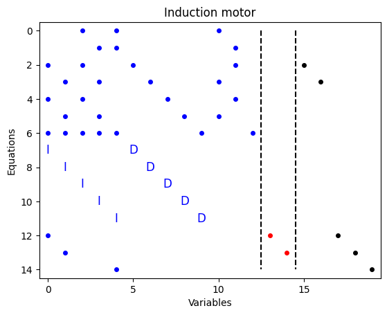
To plot the structural model, use the PlotModel class method

_, ax = plt.subplots(num=10)
model.PlotModel(ax=ax)

Basic Analysis

A basic tool in structural analysis is the Dulmage-Mendelsohn decomposition. You can perform the decomposition directly using the function fdt.dmperm.GetDMParts och using the class method GetDMParts

dm = fdt.dmperm.GetDMParts(model.X)
print(dm)
dm = model.GetDMParts()
print(dm)

DMResult(Mm=EqBlock(row=[], col=[]), M0=[EqBlock(row=array([6], dtype=int64), col=array([12], dtype=int64)), EqBlock(row=array([11], dtype=int64), col=array([9], dtype=int64))], Mp=EqBlock(row=array([ 0,  1,  2,  3,  4,  5,  7,  8,  9, 10, 12, 13, 14], dtype=int64), col=array([ 0,  1,  2,  3,  4,  5,  6,  7,  8, 10, 11], dtype=int64)), rowp=array([ 6, 11,  2,  3,  9, 10, 14,  7,  8,  4,  5,  0,  1, 12, 13],
      dtype=int64), colp=array([12,  9,  0,  1,  2,  3,  4,  5,  6,  7,  8, 10, 11], dtype=int64), M0eqs=array([ 6, 11], dtype=int64), M0vars=array([12,  9], dtype=int64))
DMResult(Mm=EqBlock(row=[], col=[]), M0=[EqBlock(row=array([6], dtype=int64), col=array([12], dtype=int64)), EqBlock(row=array([11], dtype=int64), col=array([9], dtype=int64))], Mp=EqBlock(row=array([ 0,  1,  2,  3,  4,  5,  7,  8,  9, 10, 12, 13, 14], dtype=int64), col=array([ 0,  1,  2,  3,  4,  5,  6,  7,  8, 10, 11], dtype=int64)), rowp=array([ 6, 11,  2,  3,  9, 10, 14,  7,  8,  4,  5,  0,  1, 12, 13],
      dtype=int64), colp=array([12,  9,  0,  1,  2,  3,  4,  5,  6,  7,  8, 10, 11], dtype=int64), M0eqs=array([ 6, 11], dtype=int64), M0vars=array([12,  9], dtype=int64))

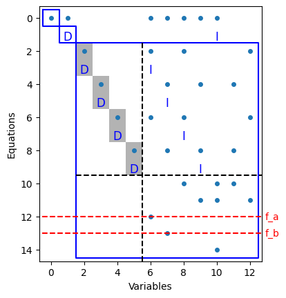
You can also visualize the decomposition using the PlotDM class method. It is also possible to do an extended Dulmage-Mendelsohn where equations are grouped in equivalence classes, see paper

Krysander, M., Åslund, J., & Nyberg, M. (2007). “An efficient algorithm for finding minimal overconstrained subsystems for model-based diagnosis”. IEEE Transactions on Systems, Man, and Cybernetics-Part A: Systems and Humans, 38(1), 197-206.

for more details.

_, ax = plt.subplots(num=23)
model.PlotDM(fault=True, eqclass=True, ax=ax)

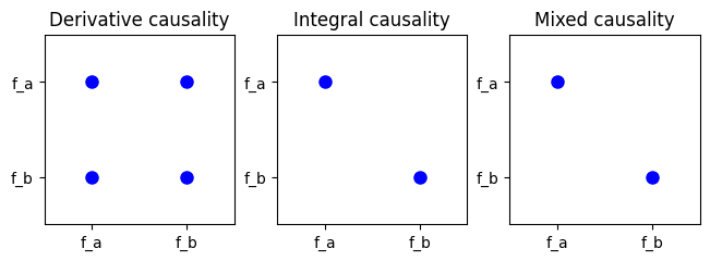
Isolability Analysis

Isolability properties of the model can be computed using the IsolabilityAnalysis method.

_, ax = plt.subplots(1, 3, num=20, layout="constrained")
model.IsolabilityAnalysis(ax=ax[0], causality='der')
model.IsolabilityAnalysis(ax=ax[1], causality='int')
model.IsolabilityAnalysis(ax=ax[2])

ax[0].set_title('Derivative causality')
ax[1].set_title('Integral causality')
ax[2].set_title('Mixed causality')

Text(0.5, 1.0, 'Mixed causality')

Redundant sets of equations

MSO and MTES sets of equations are very useful when designing residual generators. These can be directly computed using the MSO and MTES class methods as

# Find set of MSOS and MTES
msos = model.MSO()
mtes = model.MTES()
print(f"Found {len(msos)} MSO sets and {len(mtes)} MTES sets.")

Found 9 MSO sets and 2 MTES sets.

Low differential-index and observability can be directly analyzed for the MSO sets

oi_mso = [model.IsObservable(m_i) for m_i in msos]
li_mso = [model.IsLowIndex(m_i) for m_i in msos]
print(f'Out of {len(msos)} MSO sets, {sum(oi_mso)} observable, {sum(li_mso)} low (structural) differential index')

Out of 9 MSO sets, 9 observable, 4 low (structural) differential index

and also for the MTES sets

oi_mtes = [model.IsObservable(m_i) for m_i in mtes]
li_mtes = [model.IsLowIndex(m_i) for m_i in mtes]
print(f'Out of {len(mtes)} MTES sets, {sum(oi_mtes)} observable, {sum(li_mtes)} low (structural) differential index')

Out of 2 MTES sets, 2 observable, 2 low (structural) differential index

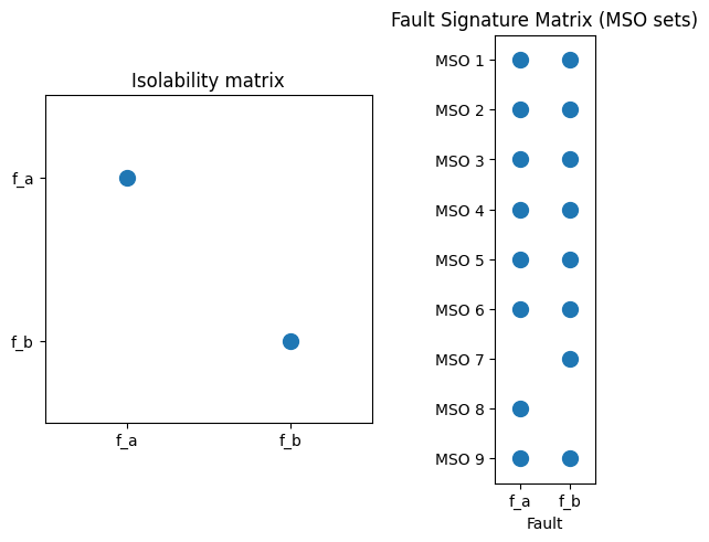
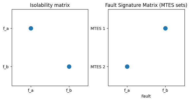
Isolability analysis for the MSO and MTES sets of equations

The isolability performance of hte full sets of MSO/MTES should be the same as the isolability performance of the model. This can be verified as below

FSM = model.FSM(msos)
fig, ax = plt.subplots(1, 2, num=30, clear=True, layout="constrained")
_ = model.IsolabilityAnalysisArrs(msos, ax=ax[0])
ax[0].set_title('Isolability matrix')

ax[1].spy(FSM, markersize=10, marker='o')
ax[1].xaxis.tick_bottom()
ax[1].set_xticks(range(model.nf()))
ax[1].set_xticklabels(model.f)
ax[1].set_yticks(range(len(msos)))
ax[1].set_yticklabels([f"MSO {i + 1}" for i in range(len(msos))])
ax[1].set_xlabel('Fault')
ax[1].set_title('Fault Signature Matrix (MSO sets)')

Text(0.5, 1.0, 'Fault Signature Matrix (MSO sets)')

FSM = model.FSM(mtes)
fig, ax = plt.subplots(1, 2, num=31, clear=True, layout="constrained")
_ = model.IsolabilityAnalysisArrs(mtes, ax=ax[0])
ax[0].set_title('Isolability matrix')

ax[1].spy(FSM, markersize=10, marker='o')
ax[1].xaxis.tick_bottom()
ax[1].set_xticks(range(model.nf()))
ax[1].set_xticklabels(model.f)
ax[1].set_yticks(range(len(mtes)))
ax[1].set_yticklabels([f"MTES {i + 1}" for i in range(len(mtes))])
ax[1].set_xlabel('Fault')
ax[1].set_title('Fault Signature Matrix (MTES sets)')

Text(0.5, 1.0, 'Fault Signature Matrix (MTES sets)')

Generate code for residual generator

Code for a residual generator, based on an MSO/MTES, can be generated. Note that this part of the toolbox is experimental and could fail at any moment.

The basic principle in sequential residual generation is to use a single equation as redundant/residual equation and use the remaining equations in the MSO/MTES to compute all unknown variables. This is done by performing a matching and then symbolically compute the analytical expressions. See below for an example.

But first, we need to determine which equation to use as a residual equation. For this, the MSOCausalitySweep is a usefuyl class method.

print(model.MSOCausalitySweep(mtes[0]))

['mixed', 'mixed', 'mixed', 'mixed', 'mixed', 'mixed', 'mixed', 'int', 'mixed', 'mixed', 'int', 'mixed']

This indicates that equations 8 and 11 results in integral causality residual generators and all other requires numerical differentiation. Let’s choose equation 11 (index 10) as redundant equation and generate the code.

red_eq = mtes[0][10]
model.syme[red_eq]
M0 = [e for e in mtes[0] if e != red_eq]

Gamma = model.Matching(M0)
model.SeqResGen(Gamma, red_eq, 'ResGen', batch=True, language='C')

Generating residual generator ResGen (C, batch)
  Generating code for the exactly determined part: ..
  Generating code for the residual equations
  Writing residual generator file
Files ResGen.cc and ResGen_setup.py generated
Compile by running: python ResGen_setup.py build_ext --inplace

It is also possible to generate Python code

model.SeqResGen(Gamma, red_eq, 'ResGen', batch=True, language='Python')

Generating residual generator ResGen (Python, batch)
  Generating code for the exactly determined part: ..
  Generating code for the residual equations
  Writing residual generator file
File ResGen.py generated.